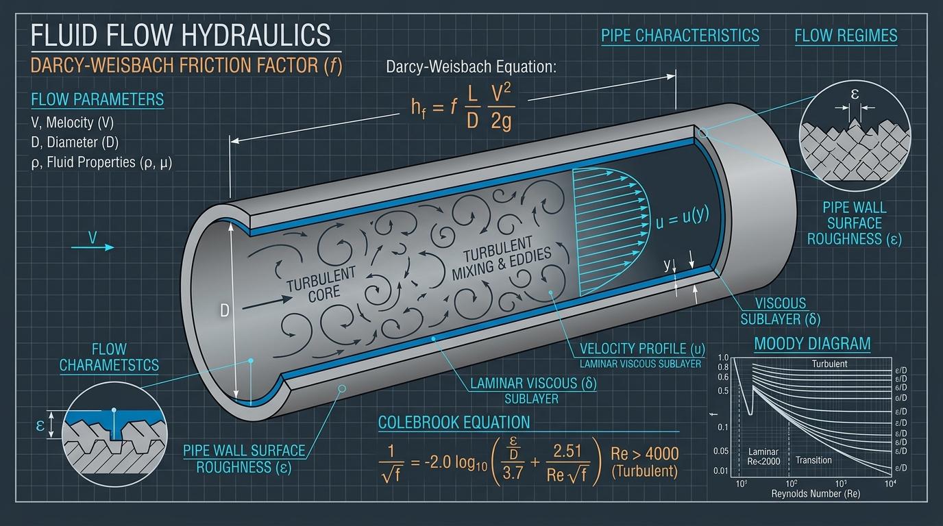
Executive Engineering Summary
Underestimating frictional head loss across industrial piping networks is among the most pervasive causes of premature pump failure, severe flow starvation, and undersized electric drive motors. While empirical formulas like Hazen-Williams remain popular in municipal waterworks, they are fundamentally inadequate for high-temperature process fluids, hydrocarbons, and viscous power plant streams. The Darcy-Weisbach formulation represents the only universally rigorous framework grounded directly in boundary layer fluid mechanics and dimensionless similitude.
1. The Governing Darcy-Weisbach Equation
Developed by Henry Darcy and Julius Weisbach, this relationship calculates continuous frictional energy dissipation along a cylindrical conduit:
Where the key variables are defined as:
- h_f:Frictional head loss in meters (or feet)
- f:Dimensionless Darcy friction factor (typically 0.012 to 0.040)
- L:Total linear straight pipe length (m or ft)
- D:Pipe internal bore diameter (m or ft)
- v:Mean cross-sectional fluid flow velocity (m/s or ft/s)
- g:Local gravitational acceleration (9.81 m/s² or 32.174 ft/s²)
2. Reynolds Number & Hydrodynamic Flow Regimes
The friction factor ($f$) is governed by the dimensionless Reynolds Number ($Re$), which quantifies the ratio of inertial forces to viscous forces in the fluid:
Laminar Flow (Re < 2,300)
Fluid moves in parallel concentric streamlines without transverse mixing. Surface roughness has zero influence on friction:
Transitional Flow (2,300 ≤ Re ≤ 4,000)
Intermittent laminar bursts transition unpredictably into turbulent eddies. Friction factors are mathematically unstable; conservative sizing adopts peak turbulent values.
Turbulent Flow (Re > 4,000)
Vigorous 3D vortex mixing dominates the flow core. The friction factor depends on both $Re$ and the relative pipe roughness ($\varepsilon/D$).
3. The Colebrook-White Equation & Swamee-Jain Approximation
In the turbulent transition and fully rough regimes, Cyril Frank Colebrook developed the celebrated implicit equation that underpins the universal Moody Chart:
Because the unknown friction factor ($f$) appears on both sides of the equation within a square root and logarithm, resolving it requires numerical iteration (such as the Newton-Raphson method). In computational software, the explicit Swamee-Jain approximation is frequently utilized, delivering ±1% accuracy for $5,000 \le Re \le 10^8$:
4. Standard Absolute Roughness Values (ε) for Industrial Materials
The physical roughness parameter $\varepsilon$ represents the mean root-mean-square height of interior wall asperities. The table below lists standard values per Hydraulic Institute and ASME standards:
| Pipe Material | Absolute Roughness ε (mm) | Absolute Roughness ε (inches) | Typical Service Life Characteristics |
|---|---|---|---|
| Commercial Carbon Steel (Schedule 40/80) | 0.045 – 0.050 mm | 0.0018 – 0.0020 in | Standard new process pipe; roughness increases with mild internal oxidation |
| Drawn Seamless Stainless Steel (304/316) | 0.015 – 0.020 mm | 0.0006 – 0.0008 in | Excellent corrosion resistance; maintains smooth boundary layer over lifetime |
| Ductile Iron (Cement Mortar Lined) | 0.025 – 0.030 mm | 0.0010 – 0.0012 in | Municipal cooling water & raw intake headers |
| Corroded / Scaled Carbon Steel Pipe | 0.150 – 0.500 mm | 0.0060 – 0.0200 in | Unbuffered steam condensate return or geothermal lines after 5+ years |
5. Summing Minor Losses: Valves, Fittings & Strainers
In compact plant layouts with extensive manifolds, minor fitting losses often exceed straight pipe friction. These losses are computed using loss resistance coefficients ($K$):
6. Detailed Step-by-Step Numerical Walkthrough
Problem: High-Pressure Water Injection Line Friction Calculation
Calculate total frictional pressure drop for water flowing at 45 m³/h (0.0125 m³/s) at 80°C (density ρ = 971.8 kg/m³, kinematic viscosity ν = 0.365 × 10⁻⁶ m²/s) through 95 meters of Schedule 40 carbon steel pipe with D = 80 mm (0.080 m, roughness ε = 0.046 mm). Fitting inventory: four 90° elbows (K=0.30 each), two gate valves (K=0.15 each), and one check valve (K=2.0).
Frequently Asked Questions: Pipe Friction & Hydraulics
Why does pipe fluid velocity matter in industrial suction piping?
High fluid velocities in pump suction lines drastically increase friction head loss, which depresses NPSHa directly. Furthermore, velocities exceeding 2.0 m/s in suction pipes generate turbulence that distorts fluid approach profiles at the impeller eye, provoking acoustic vibration and premature seal fatigue.
What is the equivalent length method for minor fitting losses?
The equivalent length method expresses minor losses in terms of an equivalent length of straight pipe that produces the identical friction drop: L_eq = (K · D) / f. Adding all L_eq values to the linear pipe length allows total loss to be evaluated in a single Darcy-Weisbach equation.
How does high fluid temperature affect pipe friction losses?
As liquid temperature increases, its dynamic viscosity drops significantly (e.g. water viscosity drops by over 70% between 20°C and 100°C). This increases the Reynolds number, driving flow deeper into the turbulent regime and slightly decreasing the friction factor f.