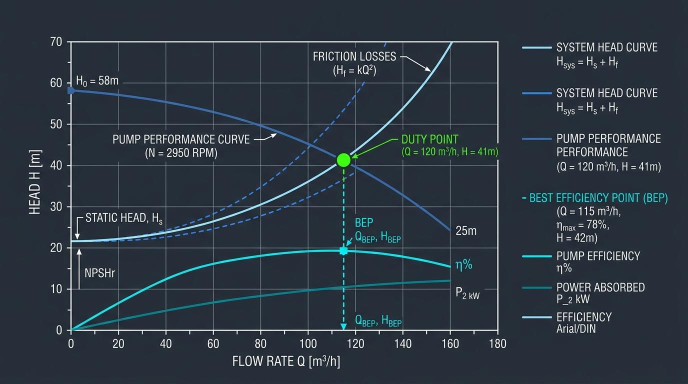
Executive Engineering Summary
In industrial fluid transport networks, centrifugal pumps do not deliver fixed flow rates or static pressures in isolation. Rather, a pump delivers fluid along a continuous performance characteristic (H_pump) dictated by its impeller blade geometry and rotational speed. The exact operating flow (Q_op) is determined exclusively where this pump curve intersects the external System Head Curve (H_sys). Misunderstanding this dynamic coupling leads to severe issues: motor overload, chronic valve erosion, cavitation damage, and massive thermodynamic inefficiencies.
1. The Anatomy of System Head: Static vs. Dynamic Resistance
Total system head represents the total mechanical energy per unit weight that the pump must impart to the fluid to transport it from the suction source to the delivery destination. Mathematically, it is divided into two distinct components:
A. Static Head Component (H_static)
Static head is completely independent of fluid velocity and volumetric flow rate (Q). It consists of:
- Static Elevation Lift (Z_geom): The net vertical elevation between suction liquid surface and destination nozzle (Z_dest - Z_source).
- Static Pressure Differential (ΔP_press): The pressure difference between the delivery vessel and the suction vessel (P_dest - P_source) converted into head units via ΔP / (ρ · g).
B. Dynamic Friction Component (H_dynamic)
Dynamic losses increase in proportion to the square of volumetric flow rate (Q²):
- Major Pipe Wall Friction: Continuous shear drag modeled via Darcy-Weisbach: h_f = f · (L/D) · (v² / 2g).
- Minor Valve & Fitting Resistance: Eddy dissipation across elbows, tees, check valves, and strainers: h_m = ∑K · (v² / 2g).
- Control Valve Pressure Drop: Differential pressure across modulating regulating valves.
2. Deriving the System Resistance Parabola (k-Factor)
Because friction head varies with velocity squared, all frictional and minor losses in a pipe system can be lumped into a single system hydraulic resistance coefficient, k_loss:
When plotting this on Cartesian coordinates with Flow (Q) on the horizontal axis and Head (H) on the vertical axis, the system curve begins at the vertical intercept (0, H_static) and arcs upward parabolically.
3. Locating the Operating Duty Point & Best Efficiency Point (BEP)
The intersection point (Q_op, H_op) where H_pump(Q) = H_system(Q) is the stable operating state of the system:
- If Flow Increases (Q > Q_op): The required system head exceeds the head the pump can produce, causing the liquid column to decelerate back to Q_op.
- If Flow Decreases (Q < Q_op): The pump head exceeds system resistance, accelerating fluid until equilibrium is restored at Q_op.
The Preferred Operating Region (POR) per ANSI/HI 9.6.3
Pumps should ideally operate between 70% and 120% of their Best Efficiency Point (BEP). Operating significantly to the left of BEP causes high radial thrust on bearings, thermal overheating from internal recirculation, and acoustic surging. Operating too far right triggers NPSHr spikes and runaway cavitation.
4. Variable Speed Control (VFD) vs. Valve Throttling Economics
When process demand calls for reduced flow, plant operators traditionally throttle a discharge control valve. While effective at shifting the system curve upward and moving the operating point to the left, throttling dissipates high pressure energy across the valve seat as noise and heat.
| Control Method | Curve Mechanism | Energy Efficiency | Mechanical Impact |
|---|---|---|---|
| VFD Speed Variation | Lowers the Pump Curve H(Q) down along Affinity Laws | Maximum (BHP drops by cube of speed: P ∝ N³) | Reduces seal wear, lowers hydraulic vibration, extends MTBF |
| Control Valve Throttling | Steepens the System Curve H_sys(Q) by artificially hiking k_loss | Poor (Dissipates surplus hydraulic energy across valve orifice) | High cavitation risk across valve seat, increased shaft deflection |
5. Comprehensive Industrial Worked Example
Problem Statement: Boiler Feed Loop System Curve
An industrial deaerator at 2.5 bar(a) supplies boiler feedwater at 125°C (density ρ = 939 kg/m³) to a boiler drum operating at 30 bar(g). Net static elevation lift is 12 meters. The suction line has 18m equivalent pipe length (D = 100 mm), and the discharge line has 160m equivalent pipe length (D = 80 mm, friction factor f = 0.019). Design flow rate is 25 m³/h (0.00694 m³/s).
Frequently Asked Questions: Pump Curves & Hydraulics
What causes a droop in a centrifugal pump curve at low flow?
A droop (or unstable curve region) occurs when the maximum head does not occur at shutoff (zero flow), but rather at some partial flow capacity. Operating a pump in this drooping region can cause hunting, severe pressure oscillations, and catastrophic surge cycles, particularly when running multiple pumps in parallel.
How do you model two pumps running in parallel versus series?
For pumps operating in parallel, flow rates add together at identical heads: Q_total = Q₁ + Q₂ at head H. For pumps operating in series (e.g. a booster pump feeding a main boiler feed pump), heads add together at identical flow rates: H_total = H₁ + H₂ at flow Q.
What is the significance of the shutoff head?
The shutoff head is the maximum total head developed by the pump when the discharge valve is completely closed (zero net flow). Centrifugal pumps typically produce 10% to 35% higher head at shutoff compared to their nominal duty point. Piping systems, flanges, and relief valves must be rated to safely withstand shutoff pressure.